Accurate Image Alignment and Registration using OpenCV

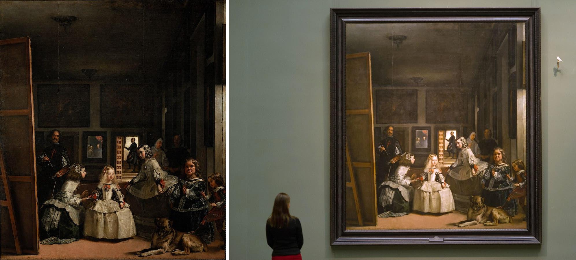
The image alignment and registration pipeline takes two input images that contain the same scene from slightly different viewing angles. The picture above displays both input images side by side with the common scene (object) being the painting Las Meninas (1656) by Velázquez, currently at the Museo del Prado in Madrid (Spain).

The first step is computing the projection that establishes the mathematical relationships which maps pixel coordinates from one image to another ¹. The most general planar 2D transformation is the eight-parameter perspective transform or homography denoted by a general $ 3×3 $ matrix $ \mathbf{H} $. It operates on 2D homogeneous coordinate vectors, $\mathbf{x’} = (x’,y’,1)$ and $\mathbf{x} = (x,y,1)$, as follows:

$$ \mathbf{x’} \sim \mathbf{Hx} $$

Afterwards, we take the homographic matrix and use it to warp the perspective of one of the images over the other, aligning the images together. With task clearly defined and the pipeline introduced, the next sections describe how this can be archieved using OpenCV.

Feature Detection

To compute the perspective transform matrix $ \mathbf{H} $, we need the link both input images and assess which regions are the same. We could manually select the corners of each painting and use that to compute the homography, however this method has several problems: the corners of a painting could be occluded in one of the scenes, not all scenes are rectangular paintings so this would not be suitable for those cases, and it would require manual work per scene, which is not ideal if want to process numerous scenes in an automatic manner.

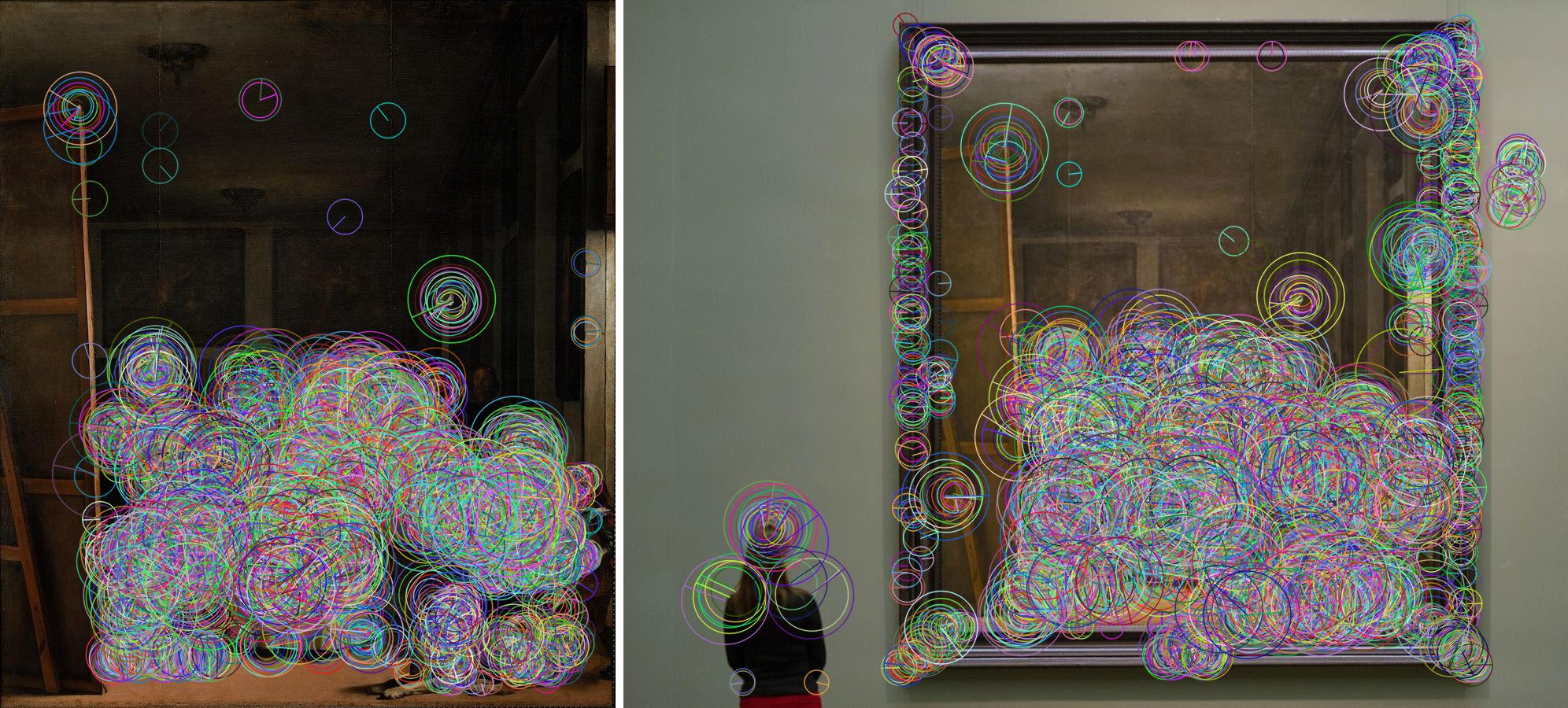
Therefore, a feature detection and matching process is used to link common regions in both images. The only limitation of this technique is that the scene must include enough features evenly distributed. The used method here was ORB ², but other feature extraction methods are also available — the code of the class FeatureExtraction is presented at the end of the post for brevity.

img0 = cv.imread("lasmeninas0.jpg", cv.COLOR_BGR2RGBA)
img1 = cv.imread("lasmeninas1.jpg", cv.COLOR_BGR2RGBA)
features0 = FeatureExtraction(img0)
features1 = FeatureExtraction(img1)

Feature Matching

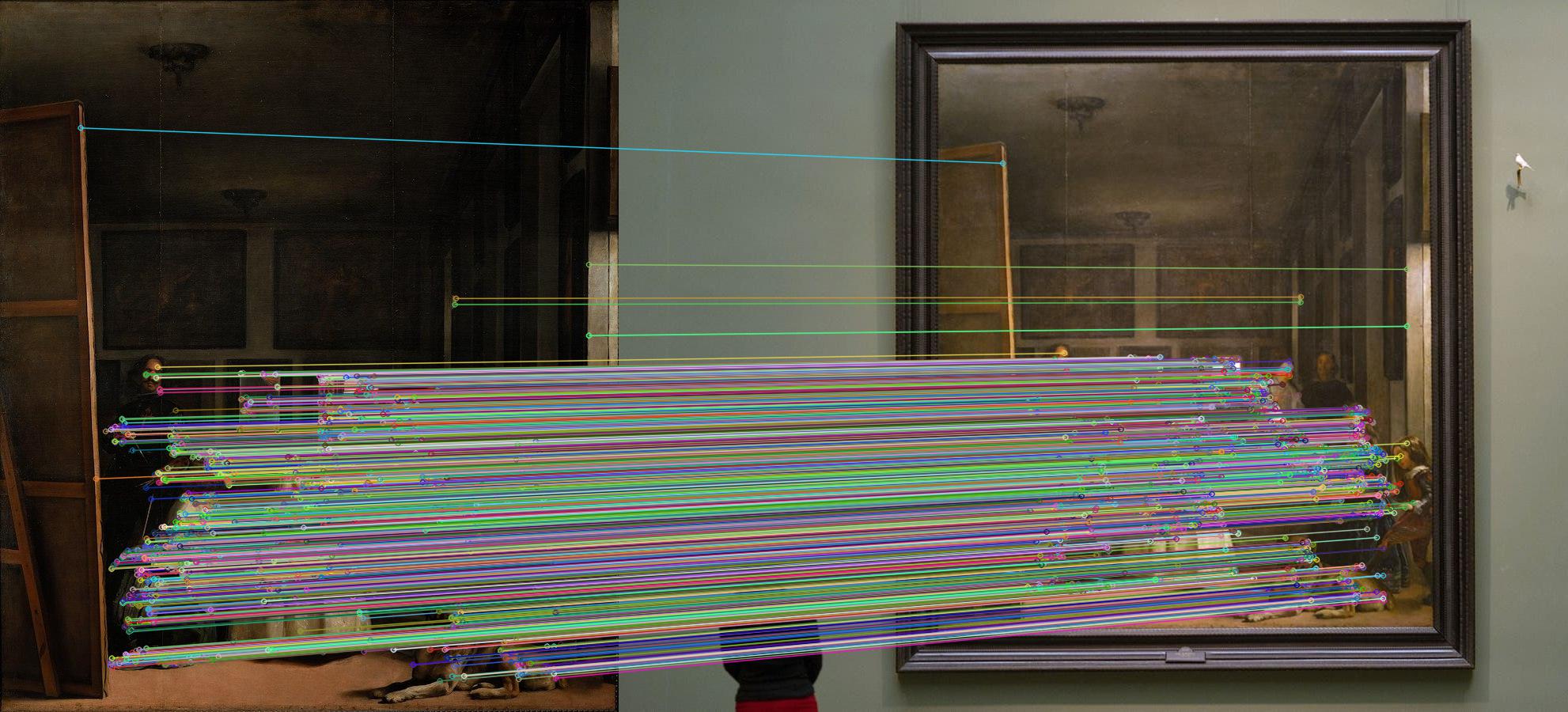
The aforementioned class computed the keypoints (position of a feature) and descriptors (description of said feature) for both images, so now we have to pair them up and remove the outliers. Firstly, FLANN (Fast Library for Approximate Nearest Neighbors) computes the pairs of matching features whilst taking into account the nearest neighbours of each feature. Secondly, the best features are selected using the Lowe’s ratio of distances test, which aims to eliminate false matches from the previous phase ³. The code is presented below, and the full function at the end. Right after the code, the picture presents both input images side by side with the matching pairs of features.

matches = feature_matching(features0, features1)
matched_image = cv.drawMatches(img0, features0.kps, \
    img1, features1.kps, matches, None, flags=2)

Homography Computation

After computing the pairs of matching features of the input images, it is possible to compute the homography matrix. It takes as input the matching points on each image and using RANSAC (random sample consensus) we are able to efficiently compute the projective matrix. Although the feature pairs were already filtered in the previous phase, they are filtered again so that only the inliers are used to compute the homography. This removes the outliers from the calculation, which leads to a minimization of the error associated with the homography computation.

H, _ = cv.findHomography( features0.matched_pts, \
    features1.matched_pts, cv.RANSAC, 5.0)

This function gives as output the following $ 3×3 $ matrix (for our input):

$$ \mathbf{H} = \begin{bmatrix} +7.85225708\text{e-}01 & -1.28373989\text{e-}02 & +4.06705815\text{e}02 \cr -4.21741196\text{e-}03 & +7.76450089\text{e-}01 & +8.15665534\text{e}01 \cr -1.20903215\text{e-}06 & -2.34464498\text{e-}05 & +1.00000000\text{e}00 \cr \end{bmatrix} $$

Perspective Warping & Overlay

Now that we have computed the transformation matrix that establishes the mathematical relationships which maps pixel coordinates from one image to another, we can do the image registration process. This process will do a perspective warp of one of the input images so that it overlaps on the other one. The outside of the warped image is filled with transparency, which then allows us to overlay that over the other image and verify its correct alignment.

h, w, c = img1.shape
warped = cv.warpPerspective(img0, H, (w, h), \
    borderMode=cv.BORDER_CONSTANT, borderValue=(0, 0, 0, 0))
output = np.zeros((h, w, 3), np.uint8)
alpha = warped[:, :, 3] / 255.0
output[:, :, 0] = (1. - alpha) * img1[:, :, 0] + alpha * warped[:, :, 0]
output[:, :, 1] = (1. - alpha) * img1[:, :, 1] + alpha * warped[:, :, 1]
output[:, :, 2] = (1. - alpha) * img1[:, :, 2] + alpha * warped[:, :, 2]

import cv2 as cv
import numpy as np
from aux import FeatureExtraction, feature_matching


img0 = cv.imread("lasmeninas0.jpg", cv.COLOR_BGR2RGBA)
img1 = cv.imread("lasmeninas1.jpg", cv.COLOR_BGR2RGBA)
features0 = FeatureExtraction(img0)
features1 = FeatureExtraction(img1)

matches = feature_matching(features0, features1)
# matched_image = cv.drawMatches(img0, features0.kps, \
#     img1, features1.kps, matches, None, flags=2)

H, _ = cv.findHomography( features0.matched_pts, \
    features1.matched_pts, cv.RANSAC, 5.0)

h, w, c = img1.shape
warped = cv.warpPerspective(img0, H, (w, h), \
    borderMode=cv.BORDER_CONSTANT, borderValue=(0, 0, 0, 0))

output = np.zeros((h, w, 3), np.uint8)
alpha = warped[:, :, 3] / 255.0
output[:, :, 0] = (1. - alpha) * img1[:, :, 0] + alpha * warped[:, :, 0]
output[:, :, 1] = (1. - alpha) * img1[:, :, 1] + alpha * warped[:, :, 1]
output[:, :, 2] = (1. - alpha) * img1[:, :, 2] + alpha * warped[:, :, 2]

import cv2 as cv
import numpy as np
import copy


orb = cv.ORB_create(
    nfeatures=10000,
    scaleFactor=1.2,
    scoreType=cv.ORB_HARRIS_SCORE)

class FeatureExtraction:
    def __init__(self, img):
        self.img = copy.copy(img)
        self.gray_img = cv.cvtColor(img, cv.COLOR_BGR2GRAY)
        self.kps, self.des = orb.detectAndCompute( \
            self.gray_img, None)
        self.img_kps = cv.drawKeypoints( \
            self.img, self.kps, 0, \
            flags=cv.DRAW_MATCHES_FLAGS_DRAW_RICH_KEYPOINTS)
        self.matched_pts = []


LOWES_RATIO = 0.7
MIN_MATCHES = 50
index_params = dict(
    algorithm = 6, # FLANN_INDEX_LSH
    table_number = 6,
    key_size = 10,
    multi_probe_level = 2)
search_params = dict(checks=50)
flann = cv.FlannBasedMatcher(
    index_params,
    search_params)

def feature_matching(features0, features1):
    matches = [] # good matches as per Lowe's ratio test
    if(features0.des is not None and len(features0.des) > 2):
        all_matches = flann.knnMatch( \
            features0.des, features1.des, k=2)
        try:
            for m,n in all_matches:
                if m.distance < LOWES_RATIO * n.distance:
                    matches.append(m)
        except ValueError:
            pass
        if(len(matches) > MIN_MATCHES):    
            features0.matched_pts = np.float32( \
                [ features0.kps[m.queryIdx].pt for m in matches ] \ 
                ).reshape(-1,1,2)
            features1.matched_pts = np.float32( \
                [ features1.kps[m.trainIdx].pt for m in matches ] \
                ).reshape(-1,1,2)
    return matches

opencv-python==4.2.0.34
numpy==1.19.2